- Design of five types of seismic force-resisting systems (SFRS) includes Special Moment Frame (SMF), Intermediate Moment Frame (IMF), Ordinary Moment Frame (OMF), Ordinary Concentrically Braced Frame (OCBF), and Special Concentrically Braced Frame (SCBF)
- Ductility check of the width-to thickness ratios for webs and flanges
- Calculation of the required strength and stiffness for stability bracing of beams
- Calculation of the maximum spacing for stability bracing of beams
- Calculation of the required strength at hinge locations for stability bracing of beams
- Calculation of the column required strength with the option to neglect all bending moments, shear, and torsion for overstrength limit state
- Design check of column and brace slenderness ratios

The building model is calculated in two phases:
- Global 3D calculation of the global model, where the slabs are modeled as a rigid plane (diaphragm) or as a bending plate
- Local 2D calculation of the individual floors
After the calculation, the results of the columns and walls from the 3D calculation and the results of the slabs from the 2D calculation are combined in a single model. This means that there is no need to switch between the 3D model and the individual 2D models of the slabs. The user only works with one model, saves valuable time, and avoids possible errors in the manual data exchange between the 3D model and the individual 2D ceiling models.
The vertical surfaces in the model can be divided into shear walls and opening lintels. The program automatically generates internal result members from these wall objects, so they can be designed as members according to any standard in the Concrete Design add-on.
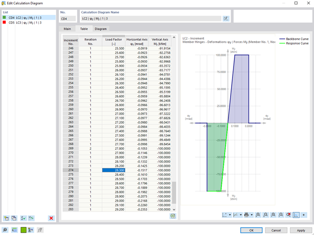
For calculation diagrams, the "2D | Hinge" is available. These hinge diagrams show the hinge response of load situations for nonlinear hinges.
For calculations with several load situations, such as is the case with pushover analyzes and time history analysis, you can evaluate the state of the hinge in each load step.
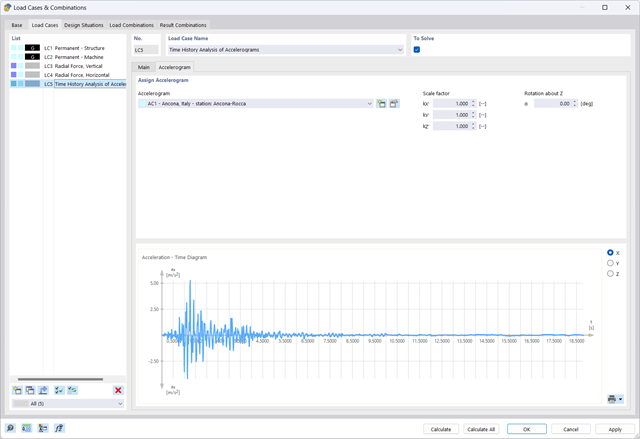
The Time History Analysis add-on provides you with accelerograms for the calculation. This extension allows for dynamic structural analysis of the acceleration-time diagrams.
There is an extensive library of earthquake records available for you, but you can also enter or import your own diagrams. The time history analysis is performed using the modal analysis or the linear implicit Newmark analysis.

The modal relevance factor (MRF) can help you to assess to which extent specific elements participate in a specific mode shape. The calculation is based on the relative elastic deformation energy of each individual member.
The MRF can be used to distinguish between local and global mode shapes. If multiple individual members show significant MRF (for example, > 20%), the instability of the entire structure or a substructure is very likely. On the other hand, if the sum of all MRFs for an eigenmode is around 100%, a local stability phenomenon (for example, buckling of a single bar) can be expected.
Furthermore, the MRF can be used to determine critical loads and equivalent buckling lengths of certain members (for example, for stability design). Mode shapes for which a specific member has small MRF values (for example, < 20%) can be neglected in this context.
The MRF is displayed by mode shape in the result table under Stability Analysis → Results by Members → Effective Lengths and Critical Loads.
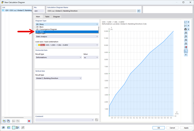
The "2D | Story" calculation diagram type is used to create result diagrams via the building axis. This allows you to easily analyze the behavior of the entire building under static and dynamic effects.
You can use this diagram type, for example, to visualize the seismic force over the building height.
- Analysis of time diagrams and accelerograms (acceleration-time diagrams exciting the supports of a structure)
- Combination of user-defined time diagrams with nodal, member, and surface loads, as well as free and generated loads
- Combination of several independent excitation functions
- Linear implicit Newmark analysis or modal analysis in time history
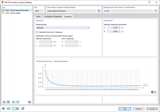
- Structural damping using Raleigh damping coefficients or Lehr's damping value
- Graphical display of results in calculation diagrams
- Result display in individual time steps or as an envelope during the entire time period
- Extensive library of seismic events (accelerograms)
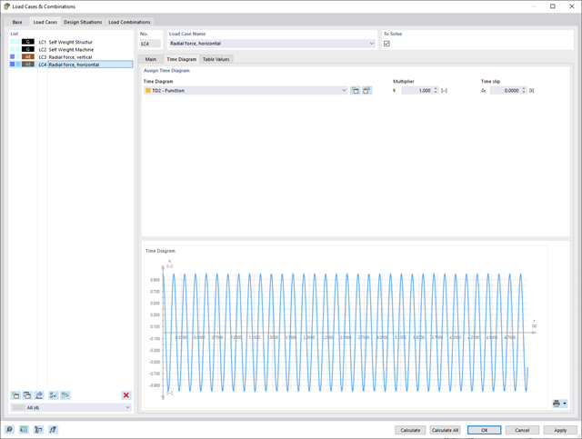
It is necessary to enter the required force-time diagrams. They can be combined in load cases or load combinations of the type Time History Analysis | Time Diagrams with the loading in order to define where and in which direction the force-time diagrams act.
The second option is to enter acceleration-time diagrams, which can be used in the load cases of the Time History Analysis | Accelerogram type.
All calculation parameters are specified in the time history analysis settings. These include, for example, the type of analysis method and the maximum calculation time.
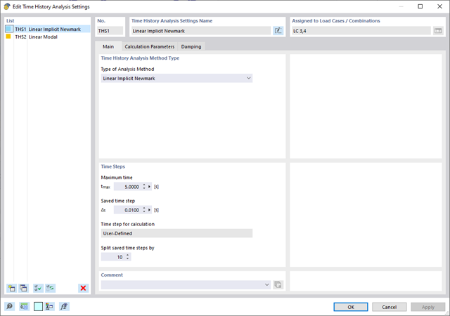
The time history analysis is performed with the modal analysis or the linear implicit Newmark analysis. The time history analysis in this add-on is limited to linear structural systems. Although the modal analysis represents a fast algorithm, it is necessary to use a certain number of eigenvalues to ensure the required accuracy of results.
The implicit Newmark analysis is a very precise method, independent of the number of eigenvalues used, but requires sufficient small time steps for the calculation.
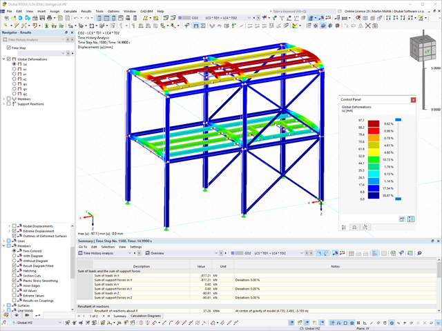
As soon as the program has completed the calculation, the summary of the results is listed. All result windows are integrated in the main program RFEM/RSTAB. You will find all the results arranged in tables; they can be displayed for each individual time step or as an envelope, and you also have the option of displaying the results graphically as well as animating them.
The results from the time history analysis can be displayed in the calculation diagrams. All the results are shown as a function of time. You can export the numeric values to MS Excel.
All result tables and graphics are part of the RFEM/RSTAB printout report. In this way, you can ensure clearly arranged documentation. You can also export the tables to MS Excel.
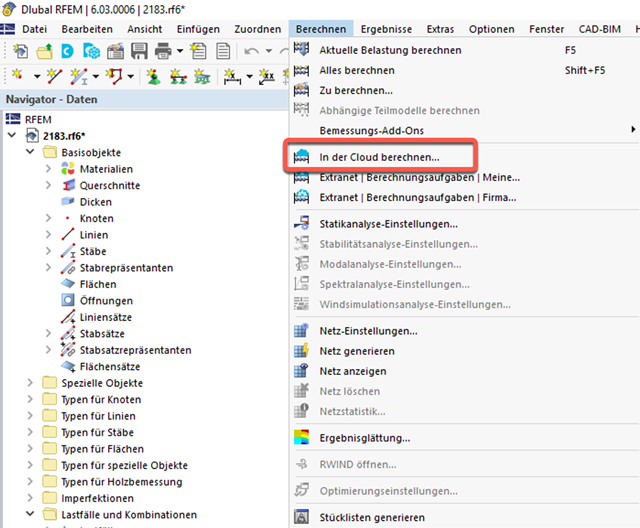
- Outsource calculation on a computing server in the cloud
- Option to select different powerful computing servers
- Clearly arranged display of all calculation tasks in the Extranet
- Calculated files are available for download for two months
- Virtually unlimited computing capacity using cloud technology
The model and loads are entered as usual in the RFEM interface.
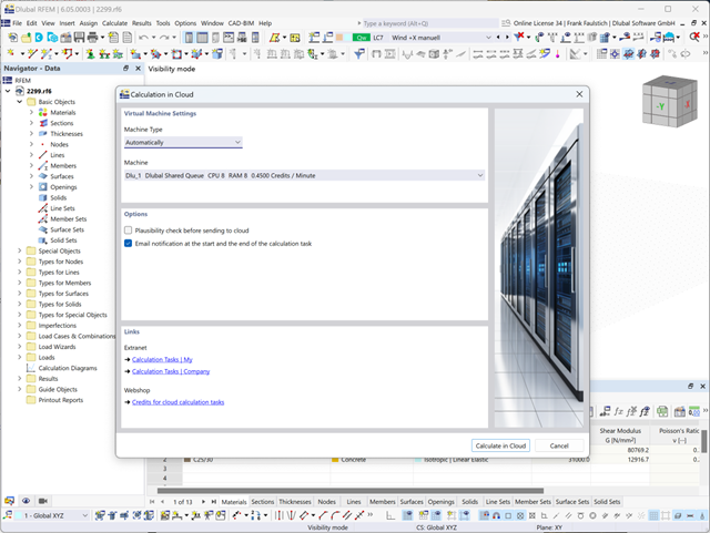
You can start the cloud calculation by selecting an entry in the Calculate menu. Then, select the virtual machine suitable for the task and start the calculation.
After the start, the image is used to create a virtual machine on which the computing server is started. This takes over the calculation of your file.
You can monitor the processing of calculation tasks in the Extranet.
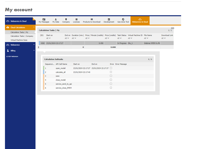
After completing the calculation, you will receive an email with a link to download the calculated file. Large files are compressed into a ZIP archive. Smaller files can be downloaded directly.
As an alternative, there is a link to the calculated file in the Extranet.
The downloaded file is a common RFEM file and can be used for further processing as usual.
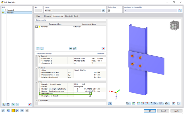
In the Steel Joints add-on, you have this option to consider the preloaded bolts in the calculation of all components.
You can easily activate the prestress using the check box in the bolt parameters, and it has an impact on the stress-strain analysis as well as the stiffness analysis.
Go to Explanatory Video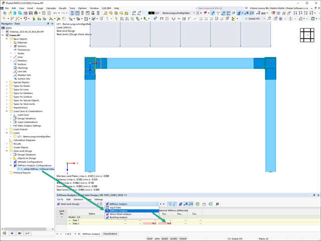
In the Steel Joints add-on, you can determine the initial stiffness Sj,ini according to Eurocode and AISC. This can be done for selected members with reference to the internal forces N, My, and Mz.
In the Members tab of the input dialog box of the Steel Joints add-on, you can select the desired internal forces via a checkbox. Multiple selection is possible. For these internal forces, the stiffness analysis is carried out with a positive and a negative sign.
Go to Explanatory Video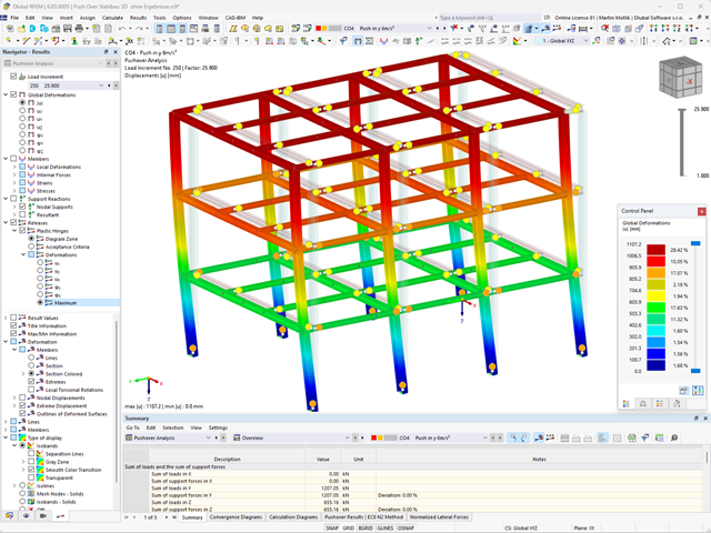
- Consideration of nonlinear component behavior using plastic standard hinges for steel (FEMA 356, EN 1998‑3) and nonlinear material behavior (masonry, steel - bilinear, user-defined working curves)
- Direct import of masses from load cases or combinations for the application of constant vertical loads
- User-defined specifications for the consideration of horizontal loads (standardized to a mode shape or uniformly distributed over the height of the masses)
- Determination of a pushover curve with selectable limit criterion of the calculation (a collapse or limit deformation)
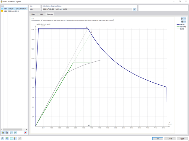
- Transformation of the pushover curve into the capacity spectrum (ADRS format, single degree of freedom system)
- Bilinearization of the capacity spectrum according to EN 1998‑1:2010 + A1:2013
- Transformation of the applied response spectrum into the required spectrum (ADRS format)
- Determination of target displacement according to EC 8 (the N2 method according to Fajfar 2000)
- Graphical comparison of the capacity and required spectrum
- Graphical evaluation of the acceptance criteria of predefined plastic hinges
- Result display of the values used in the iterative calculation of the target displacement
- Access to all results of the structural analysis in the individual load levels
During the calculation, the selected horizontal load is increased in load steps. A static nonlinear analysis is carried out for each load step until reaching the specified limit condition.
The results of the pushover analysis are extensive. On one hand, the structure is analyzed for its deformation behavior. This can be represented by a force-deformation line of the system (a capacity curve). On the other hand, the response spectrum effect can be displayed in the ADRS display (Acceleration-Displacement Response Spectrum). The target displacement is automatically determined in the program based on these two results. The process can be evaluated graphically and in tables.
The individual acceptance criteria can then be graphically evaluated and assessed (for the next load step of the target displacement, but also for all other load steps). The results of the static analysis are also available for the individual load steps.
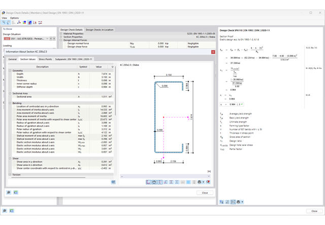
Would you like to perform cross-section design checks for cold-formed steel members according to EN 1993‑1‑3? No matter if you design the cold-formed sections from the cross-section library or the general cold-formed (non-perforated) sections from RSECTION – your structural analysis program helps you to determine the effective cross-section, taking into account the local buckling and instability. You can also perform a cross-section check according to EN 1993‑1‑3, 6.1.6. In this case, the internal forces from the calculation using Torsional Warping (7 DOF) are taken into account by means of the equivalent stress check
Go to Explanatory Video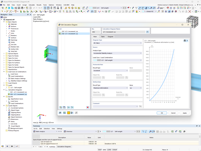
Do you want to create calculation diagrams? With RFEM and RSTAB, this works globally and without any problems. Create and organize your calculation diagrams directly in the Navigator - Data or via the menu Insert → Calculation Diagrams.
Use calculation diagrams to record and display a relation between the various calculation results.
It is also possible to superimpose similar diagrams.
The Torsional Warping (7 DOF) add-on allows you to perform the calculation of member structures in RFEM and RSTAB, taking into account the cross-section warping. You can consider all internal forces (N, Vu, Vv, Mt,pri, Mt,sec, Mu, Mv, Mω) determined in this way in the equivalent stress analysis of the aluminum design. Please Note: This feature is not yet available for the design standard ADM 2020.

Are you ready for the evaluation? Use the calculation diagrams, which show the distribution of a specific result during the calculation.
You can freely define the layout of the vertical and horizontal axes of the calculation diagram. This allows you, for example, to consider the settlement distribution of a certain node, depending on the load.
- Calculation of deflections and comparison with the normative or manually adjusted limit values
- Consideration of a precamber for the deflection analysis
- Different limit values are possible, depending on the design situation type
- Manual Adjustment of Reference Lengths and Segmentation by Direction
- Calculation of deflections related to the initial structure or to the deformed structure
- Further detailed design checks depending on the selected design standard (for example, vibration design according to EN 1999‑1‑1, 7.2.3)
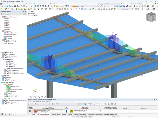
- Graphical result display integrated in RFEM/RSTAB; for example, the design ratio of a limit value, or the deformation or the sag
- Complete integration of the results into the RFEM/RSTAB printout report
You can find the serviceability limit state design checks in the result tables of the Aluminum Design add-on. They are already fully integrated there. You have the option to display the design results with all the details at each location of the designed members. You can also use graphics with the result diagrams of the design ratios.
You can integrate all result tables and graphics into the global printout report of RFEM/RSTAB as a part of the aluminum design results. RFEM/RSTAB also allows you to display and document the deformations of the entire structure independently of the add-on.
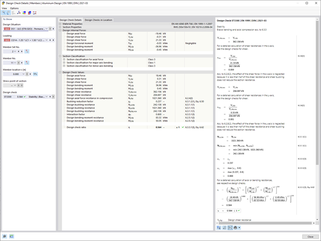
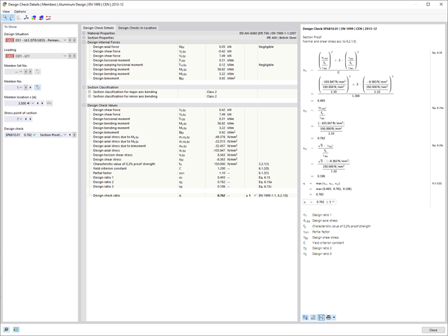
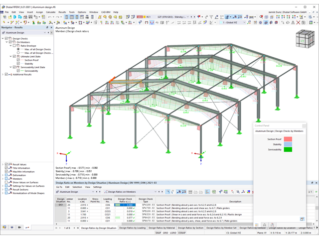
Do you prefer it clear? So do we! That's why all performed design checks for the design standard are displayed for you in a clear way. You determine a design criterion for each design check. You get design details, which include the initial values, intermediate results, and final results, arranged in a structured way for each design check. You can find the calculation process with the applied formulas, standard sources, and results in great detail in an information window in the design details.
As usual, you enter the structural system and calculate the internal forces in the programs RFEM and RSTAB. You have unlimited access to the extensive material and cross-section libraries. Did you know that you can create general cross-sections using the RSECTION program? That saves you a lot of work.
Don't be afraid of additional windows and input chaos! Aluminum Design is completely integrated into the main programs and automatically takes into account the structure and the available calculation results. You can directly assign further entries for the aluminum design, such as effective lengths, cross-section reductions, or design parameters, to the objects to be designed. You can simply and efficiently select the elements graphically using the [Select] function.

Enter and model a soil solid directly in RFEM. You can combine the soil material models with all common RFEM add-ons.
This allows you to easily analyze the entire models with a complete representation of the soil-structure interaction.
All parameters required for the calculation are automatically determined from the material data that you have entered. The program then generates the stress-strain curves for each FE element.

As you've already learned, the results of a Modal Analysis load case are displayed in the program after a successful calculation. You can thus immediately see the first mode shape graphically or as an animation. You can also easily adjust the representation of the mode shape standardization. Do that directly in the Results navigator, where you have one of four options for the visualization of the mode shapes available for the selection:
- Scaling the value of the mode shape vector uj to 1 (considers the translation components only)
- Selecting the maximum translational component of the eigenvector and setting it to 1
- Considering the entire eigenvector (including the rotation components), selecting the maximum, and setting it to 1
- Setting the modal mass mi for each mode shape to 1 kg
You can find a detailed explanation of the mode shape standardization in the OnlineManual here.

It is often necessary to neglect masses. This is particularly the case when you want to use the output of the modal analysis for the seismic analysis. For this, 90% of the effective modal mass in each direction is required for the calculation. So you can neglect the mass in all fixed nodal and line supports. The program automatically deactivates the associated masses for you.
You can also manually select the objects whose masses are to be neglected for the modal analysis. We have shown the latter in the image for a better view. A user-defined selection is made the and the objects with their associated mass components are selected to neglect the masses.

Is the calculation finished? The results of the modal analysis are then available both graphically and in tables. Display the result tables for the load case or the load cases of the modal analysis. Thus, you can see the eigenvalues, angular frequencies, natural frequencies, and natural periods of the structure at first glance. The effective modal masses, modal mass factors, and participation factors are also clearly displayed.

RFEM allows you to use a special line hinge to model the special properties of the connection between the reinforced concrete slab and masonry wall. This limits the transferable forces of the connection depending on the specified geometry. You guess right: This means that the material cannot be overloaded.
The program develops interaction diagrams that are applied automatically. They represent the various geometric situations and you can use them to determine the correct stiffness.